from: https://blog.auberginesolutions.com/scratching-the-surface-of-generative-adversarial-networks/
In this article, we’ll try to understand how computers of today are able to generate fake faces more precisely than any human with the help of GANs.
Generative Adversarial Networks(GANs) are a type of generative modeling with deep neural networks like Convolutional Neural Networks(CNNs).
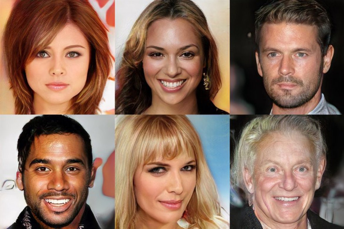
GANs are the type of Unsupervised learning that includes recognizing patterns from an image and generating fake images similar to real ones. These fake images look so real that even humans can’t differentiate between them. Below images are generated using the GAN algorithm and these people are not real.
How GAN works?
GANs have two different types of neural networks:
- Generator to generate a fake image from noisy data
- Discriminator to distinguish between the real image and fake image.
Its structural representation is as follows:
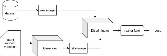
Here, the job of the discriminator is to estimate the probability that the sample came from training data rather than the generator. And the generator tries to maximize the chances of discriminator being wrong. So, this looks similar to two players in a min-max game where each of them is trying to beat each other while improving themselves. At the end of the training, generated data from the generator will have the same distribution as training data and the probability of discriminator will stick to 1/2. This entire system is based on the concept of backpropagation. So, there’s no need for Markov Chains or inference during the generation of images.
Theory
The generator’s job is to learn distribution Pg over training data x, so the input noise variable is Pz(Z). So, the generator’s mapping to data space representation is G(z; θg) where G is a neural network with parameters θg. A second neural network is Discriminator with D(x, θd) which outputs a single scalar value. D(x) represents the probability that x came from the data rather than Pg.
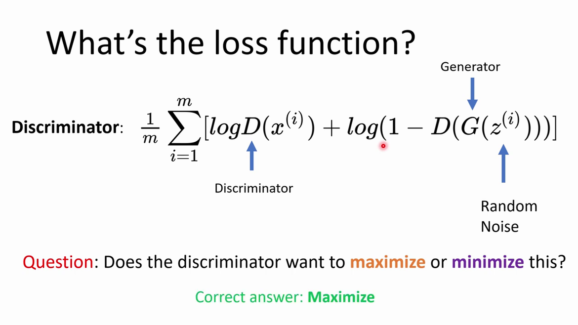
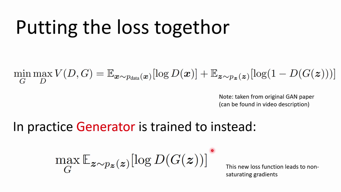
As shown in the structural diagram, the results from discriminator will be fed to the loss function. This loss function is as follows:

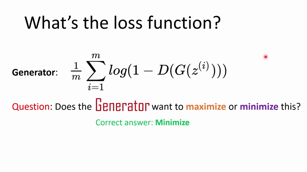
Here the job of the discriminator is to maximize the probability of assigning the correct label and train generator to minimize log(1-D(G(z))).
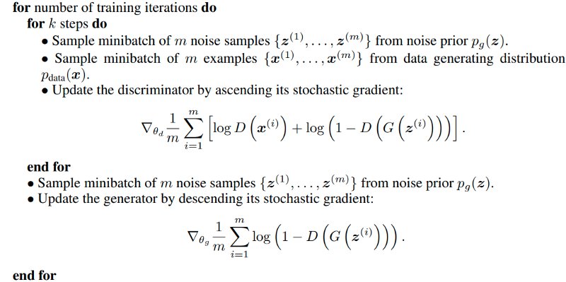
One important thing to keep in mind is that both these networks should be well balanced while training so none of them is overfitted. So after every k steps of optimizing the discriminator, the generator will optimize once. This results in D being maintained near its optimal solution, so long as G changes slowly enough.
Visualizing training process
Now let’s see how this GAN training process looks in visualizations.
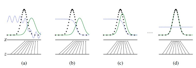
In the above diagram, the blue dotted line represents discriminator, black dotted line represents training data distribution and the green solid line represents generator distribution. The horizontal line below represents the domain from which input z is sampled for generator and above horizontal line represents the domain of training data x.
Figure (a) shows the starting of the process and Figure (d) is the end of the process. The distribution of the generator input is similar to training data distribution.
Algorithm
Advantages and Disadvantages
Advantages
- It does not use Markov Chains or inference.
- Instead, it only requires Backpropagation.
- It incorporates a wide variety of functions.
- It doesn’t update from data directly but instead uses feedback from a discriminator.
Disadvantages
- There is no explicit representation of distribution of generator data (Pg)
- Discriminators and Generators must be synced well with each other during training i.e. none of the networks should over power each other.
Conclusion
As we discussed earlier, GANs are simple generative algorithms with two multilayer perceptions. For diving deeper into GANs, please refer to this paper.
In the next article, we’ll try to understand how to implement simple Generative Adversarial Network using python.