Machines are generating perfect images these days and it’s becoming more and more difficult to distinguish the machine-generated images from the originals.
If you are reading this article, I am sure that we share similar interests and are/will be in similar industries. So let’s connect via Linkedin! Please do not hesitate to send a contact request! Orhan G. Yalçın — Linkedin

After receiving more than 300k views for my article, Image Classification in 10 Minutes with MNIST Dataset, I decided to prepare another tutorial on deep learning. But this time, instead of classifying images, we will generate images using the same MNIST dataset, which stands for Modified National Institute of Standards and Technology database. It is a large database of handwritten digits that is commonly used for training various image processing systems[1].
Generative Adversarial Networks
To generate -well basically- anything with machine learning, we have to use a generative algorithm and at least for now, one of the best performing generative algorithms for image generation is Generative Adversarial Networks (or GANs).
The invention of Generative Adversarial Network
The invention of GANs has occurred pretty unexpectedly. The famous AI researcher, then, a Ph.D. fellow at the University of Montreal, Ian Goodfellow, landed on the idea when he was discussing with his friends -at a friend’s going away party- about the flaws of the other generative algorithms. After the party, he came home with high hopes and implemented the concept he had in mind. Surprisingly, everything went as he hoped in the first trial [5] and he successfully created the Generative Adversarial Networks (shortly, GANs). According to Yann Lecun, the director of AI research at Facebook and a professor at New York University, GANs are “the most interesting idea in the last 10 years in machine learning” [6].
The rough structure of the GANs may be demonstrated as follows:
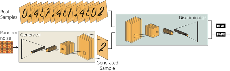
In an ordinary GAN structure, there are two agents competing with each other: a Generator and a Discriminator. They may be designed using different networks (e.g. Convolutional Neural Networks (CNNs), Recurrent Neural Networks (RNNs), or just Regular Neural Networks (ANNs or RegularNets)). Since we will generate images, CNNs are better suited for the task. Therefore, we will build our agents with convolutional neural networks.
How does our GAN model operate?
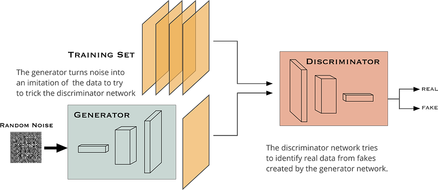
In a nutshell, we will ask the generator to generate handwritten digits without giving it any additional data. Simultaneously, we will fetch the existing handwritten digits to the discriminator and ask it to decide whether the images generated by the Generator are genuine or not. At first, the Generator will generate lousy images that will immediately be labeled as fake by the Discriminator. After getting enough feedback from the Discriminator, the Generator will learn to trick the Discriminator as a result of the decreased variation from the genuine images. Consequently, we will obtain a very good generative model which can give us very realistic outputs.
Building the GAN Model
GANs often use computationally complex calculations and therefore, GPU-enabled machines will make your life a lot easier. Therefore, I will use Google Colab to decrease the training time with GPU acceleration.
GPU-Enabled Training with Google Colab
For machine learning tasks, for a long time, I used to use -iPython- Jupyter Notebook via Anaconda distribution for model building, training, and testing almost exclusively. Lately, though, I have switched to Google Colab for several good reasons.
Google Colab offers several additional features on top of the Jupyter Notebook such as (i) collaboration with other developers, (ii) cloud-based hosting, and (iii) GPU & TPU accelerated training. You can do all these with the free version of Google Colab. The relationship between Python, Jupyter Notebook, and Google Colab can be visualized as follows:
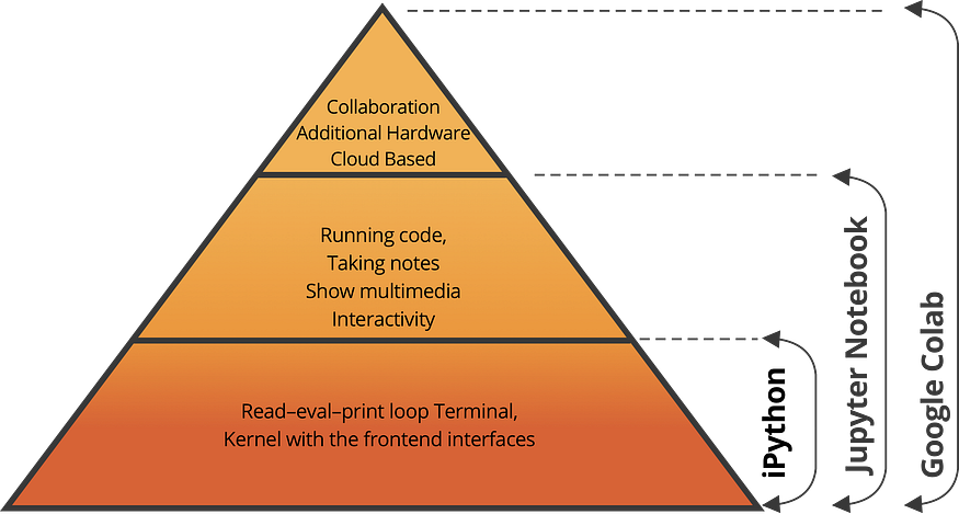
Anaconda provides free and open-source distribution of the Python and R programming languages for scientific computing with tools like Jupyter Notebook (iPython) or Jupyter Lab. On top of these tools, Google Colab lets its users use the iPython notebook and lab tools with the computing power of their servers.
Now that we have a general understanding of generative adversarial networks as our neural network architecture and Google Collaboratory as our programming environment, we can start building our model. In this tutorial, we will do our own take from an official TensorFlow tutorial [7].
Initial Imports
Colab already has most machine learning libraries pre-installed, and therefore, you can just import them as shared below:
import tensorflow as tf
from tensorflow.keras.layers import (Dense,
                                     BatchNormalization,
                                     LeakyReLU,
                                     Reshape,
                                     Conv2DTranspose,
                                     Conv2D,
                                     Dropout,
                                     Flatten)
import matplotlib.pyplot as plt
For the sake of shorter code, I prefer to import layers individually, as shown above.
Load and Process the MNIST Dataset
For this tutorial, we can use the MNIST dataset. The MNIST dataset contains 60,000 training images and 10,000 testing images taken from American Census Bureau employees and American high school students [8].
Luckily we may directly retrieve the MNIST dataset from the TensorFlow library. We retrieve the dataset from Tensorflow because this way, we can have the already processed version of it. We still need to do a few preparation and processing works to fit our data into the GAN model. Therefore, in the second line, we separate these two groups as train and test and also separated the labels and the images.
x_train and x_test parts contain greyscale RGB codes (from 0 to 255) while y_train and y_test parts contain labels from 0 to 9 which represents which number they actually are. Since we are doing an unsupervised learning task, we will not need label values and therefore, we use underscores (i.e., _) to ignore them. We also need to convert our dataset to 4-dimensions with the reshape function. Finally, we convert our NumPy array to a TensorFlow Dataset object for more efficient training. The lines below do all these tasks:
# underscore to omit the label arrays
(train_images, train_labels), (_, _) = tf.keras.datasets.mnist.load_data()


train_images = train_images.reshape(train_images.shape[0], 28, 28, 1).astype('float32')
train_images = (train_images - 127.5) / 127.5 # Normalize the images to [-1, 1]

BUFFER_SIZE = 60000
BATCH_SIZE = 256

# Batch and shuffle the data
train_dataset = tf.data.Dataset.from_tensor_slices(train_images).shuffle(BUFFER_SIZE).batch(BATCH_SIZE)
Our data is already processed and it is time to build our GAN model.
Build the Model
As mentioned above, every GAN must have at least one generator and one discriminator. Since we are dealing with image data, we need to benefit from Convolution and Transposed Convolution (Inverse Convolution) layers in these networks. Let's define our generator and discriminator networks below.
Generator Network
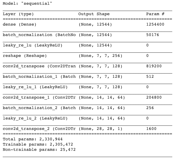
Our generator network is responsible for generating 28x28 pixels grayscale fake images from random noise. Therefore, it needs to accept 1-dimensional arrays and output 28x28 pixels images. For this task, we need Transposed Convolution layers after reshaping our 1-dimensional array to a 2-dimensional array. Transposed Convolution layers can increase the size of a smaller array. We also take advantage of BatchNormalization and LeakyReLU layers. The below lines create a function which would generate a generator network with Keras Sequential API:
def make_generator_model():
    model = tf.keras.Sequential()
    model.add(Dense(7*7*256, use_bias=False, input_shape=(100,)))
    model.add(BatchNormalization())
    model.add(LeakyReLU())

    model.add(Reshape((7, 7, 256)))
    assert model.output_shape == (None, 7, 7, 256) # Note: None is the batch size

    model.add(Conv2DTranspose(128, (5, 5), strides=(1, 1), padding='same', use_bias=False))
    assert model.output_shape == (None, 7, 7, 128)
    model.add(BatchNormalization())
    model.add(LeakyReLU())

    model.add(Conv2DTranspose(64, (5, 5), strides=(2, 2), padding='same', use_bias=False))
    assert model.output_shape == (None, 14, 14, 64)
    model.add(BatchNormalization())
    model.add(LeakyReLU())

    model.add(Conv2DTranspose(1, (5, 5), strides=(2, 2), padding='same', use_bias=False, activation='tanh'))
    assert model.output_shape == (None, 28, 28, 1)

    return model
We can call our generator function with the following code:
generator = make_generator_model()
Now that we have our generator network, we can easily generate a sample image with the following code:
# Create a random noise and generate a sample
noise = tf.random.normal([1, 100])
generated_image = generator(noise, training=False)
# Visualize the generated sample
plt.imshow(generated_image[0, :, :, 0], cmap='gray')
which would look like this:
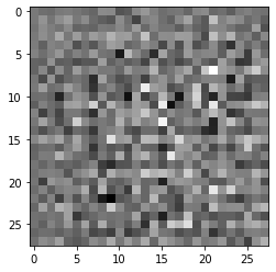
It is just plain noise. But, the fact that it can create an image from a random noise array proves its potential.
Discriminator Network
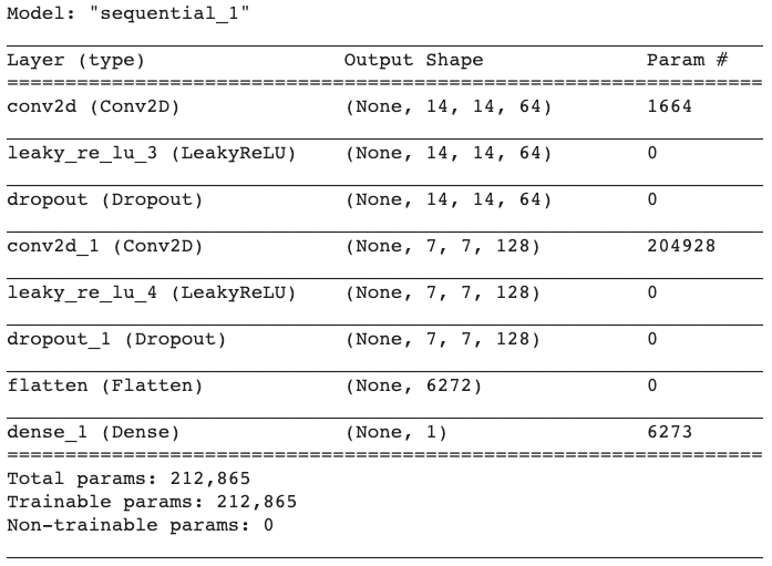
For our discriminator network, we need to follow the inverse version of our generator network. It takes the 28x28 pixels image data and outputs a single value, representing the possibility of authenticity. So, our discriminator can review whether a sample image generated by the generator is fake.
We follow the same method that we used to create a generator network, The following lines create a function that would create a discriminator model using Keras Sequential API:
def make_discriminator_model():
    model = tf.keras.Sequential()

    model.add(Conv2D(64, (5, 5), strides=(2, 2), padding='same', input_shape=[28, 28, 1]))
    model.add(LeakyReLU())
    model.add(Dropout(0.3))

    model.add(Conv2D(128, (5, 5), strides=(2, 2), padding='same'))
    model.add(LeakyReLU())
    model.add(Dropout(0.3))

    model.add(Flatten())
    model.add(Dense(1))

    return model
We can call the function to create our discriminator network with the following line:
discriminator = make_discriminator_model()
Finally, we can check what our non-trained discriminator says about the sample generated by the non-trained generator:
decision = discriminator(generated_image)
print (decision)
Output: tf.Tensor([[-0.00108097]], shape=(1, 1), dtype=float32)
A negative value shows that our non-trained discriminator concludes that the image sample in Figure 8 is fake. At the moment, what's important is that it can examine images and provide results, and the results will be much more reliable after training.
Configure the Model
Since we are training two sub-networks inside a GAN network, we need to define two loss functions and two optimizers.
Loss Functions: We start by creating a Binary Crossentropy object from tf.keras.losses module. We also set the from_logits parameter to True. After creating the object, we fill them with custom discriminator and generator loss functions. Our discriminator loss is calculated as a combination of (i) the discriminator’s predictions on real images to an array of ones and (ii) its predictions on generated images to an array of zeros. Our generator loss is calculated by measuring how well it was able to trick the discriminator. Therefore, we need to compare the discriminator’s decisions on the generated images to an array of 1s.
Optimizers: We also set two optimizers separately for generator and discriminator networks. We can use the Adam optimizer object from tf.keras.optimizers module.
The following lines configure our loss functions and optimizers
# This method returns a helper function to compute cross entropy loss
cross_entropy = tf.keras.losses.BinaryCrossentropy(from_logits=True)

def discriminator_loss(real_output, fake_output):
    real_loss = cross_entropy(tf.ones_like(real_output), real_output)
    fake_loss = cross_entropy(tf.zeros_like(fake_output), fake_output)
    total_loss = real_loss + fake_loss
    return total_loss

def generator_loss(fake_output):
    return cross_entropy(tf.ones_like(fake_output), fake_output)

generator_optimizer = tf.keras.optimizers.Adam(1e-4)
discriminator_optimizer = tf.keras.optimizers.Adam(1e-4)
Set the Checkpoints
We would like to have access to previous training steps and TensorFlow has an option for this: checkpoints. By setting a checkpoint directory, we can save our progress at every epoch. This will be especially useful when we restore our model from the last epoch. The following lines configure the training checkpoints by using the os library to set a path to save all the training steps
import os

checkpoint_dir = './training_checkpoints'
checkpoint_prefix = os.path.join(checkpoint_dir, "ckpt")
checkpoint = tf.train.Checkpoint(generator_optimizer=generator_optimizer,
                                 discriminator_optimizer=discriminator_optimizer,
                                 generator=generator,
                                 discriminator=discriminator)
Train the Model
Now our data ready, our model is created and configured. It is time to design our training loop. Note that at the moment, GANs require custom training loops and steps. I will try to make them as understandable as possible for you. Make sure that you read the code comments in the Github Gists.
Let’s create some of the variables with the following lines:
EPOCHS = 60
# We will reuse this seed overtime (so it's easier)
# to visualize progress in the animated GIF)
num_examples_to_generate = 16
noise_dim = 100
seed = tf.random.normal([num_examples_to_generate, noise_dim])
Our seed is the noise that we use to generate images on top of. The code below generates a random array with normal distribution with the shape (16, 100).
Define the Training Step
This is the most unusual part of our tutorial: We are setting a custom training step. After defining the custom train_step() function by annotating the tf.function module, our model will be trained based on the custom train_step() function we defined.
The code below with excessive comments are for the training step. Please read the comments carefully:
# tf.function annotation causes the function
# to be "compiled" as part of the training
@tf.function
def train_step(images):

    # 1 - Create a random noise to feed it into the model
    # for the image generation
    noise = tf.random.normal([BATCH_SIZE, noise_dim])

    # 2 - Generate images and calculate loss values
    # GradientTape method records operations for automatic differentiation.
    with tf.GradientTape() as gen_tape, tf.GradientTape() as disc_tape:
      generated_images = generator(noise, training=True)

      real_output = discriminator(images, training=True)
      fake_output = discriminator(generated_images, training=True)

      gen_loss = generator_loss(fake_output)
      disc_loss = discriminator_loss(real_output, fake_output)

    # 3 - Calculate gradients using loss values and model variables
    # "gradient" method computes the gradient using
    # operations recorded in context of this tape (gen_tape and disc_tape).

    # It accepts a target (e.g., gen_loss) variable and
    # a source variable (e.g.,generator.trainable_variables)
    # target --> a list or nested structure of Tensors or Variables to be differentiated.
    # source --> a list or nested structure of Tensors or Variables.
    # target will be differentiated against elements in sources.

    # "gradient" method returns a list or nested structure of Tensors
    # (or IndexedSlices, or None), one for each element in sources.
    # Returned structure is the same as the structure of sources.
    gradients_of_generator = gen_tape.gradient(gen_loss,
                                               generator.trainable_variables)
    gradients_of_discriminator = disc_tape.gradient(disc_loss,
                                                discriminator.trainable_variables)

    # 4 - Process  Gradients and Run the Optimizer
    # "apply_gradients" method processes aggregated gradients.
    # ex: optimizer.apply_gradients(zip(grads, vars))
    """
    Example use of apply_gradients:
    grads = tape.gradient(loss, vars)
    grads = tf.distribute.get_replica_context().all_reduce('sum', grads)
    # Processing aggregated gradients.
    optimizer.apply_gradients(zip(grads, vars), experimental_aggregate_gradients=False)
    """
    generator_optimizer.apply_gradients(zip(gradients_of_generator, generator.trainable_variables))
    discriminator_optimizer.apply_gradients(zip(gradients_of_discriminator, discriminator.trainable_variables))
Now that we created our custom training step with tf.function annotation, we can define our train function for the training loop.
Define the Training Loop
We define a function, named train, for our training loop. Not only we run a for loop to iterate our custom training step over the MNIST, but also do the following with a single function:
During the Training:
- Start recording time spent at the beginning of each epoch;
- Produce GIF images and display them,
- Save the model every five epochs as a checkpoint,
- Print out the completed epoch time; and
- Generate a final image in the end after the training is completed.
The following lines with detailed comments, do all these tasks:
import time
from IPython import display # A command shell for interactive computing in Python.

def train(dataset, epochs):
  # A. For each epoch, do the following:
  for epoch in range(epochs):
    start = time.time()
    # 1 - For each batch of the epoch,
    for image_batch in dataset:
      # 1.a - run the custom "train_step" function
      # we just declared above
      train_step(image_batch)

    # 2 - Produce images for the GIF as we go
    display.clear_output(wait=True)
    generate_and_save_images(generator,
                             epoch + 1,
                             seed)

    # 3 - Save the model every 5 epochs as
    # a checkpoint, which we will use later
    if (epoch + 1) % 5 == 0:
      checkpoint.save(file_prefix = checkpoint_prefix)

    # 4 - Print out the completed epoch no. and the time spent
    print ('Time for epoch {} is {} sec'.format(epoch + 1, time.time()-start))

  # B. Generate a final image after the training is completed
  display.clear_output(wait=True)
  generate_and_save_images(generator,
                           epochs,
                           seed)
Image Generation Function
In the train function, there is a custom image generation function that we haven’t defined yet. Our image generation function does the following tasks:
- Generate images by using the model;
- Display the generated images in a 4x4 grid layout using matplotlib;
- Save the final figure in the end
The following lines are in charge of these tasks:
def generate_and_save_images(model, epoch, test_input):
  # Notice `training` is set to False.
  # This is so all layers run in inference mode (batchnorm).
  # 1 - Generate images
  predictions = model(test_input, training=False)
  # 2 - Plot the generated images
  fig = plt.figure(figsize=(4,4))
  for i in range(predictions.shape[0]):
      plt.subplot(4, 4, i+1)
      plt.imshow(predictions[i, :, :, 0] * 127.5 + 127.5, cmap='gray')
      plt.axis('off')
  # 3 - Save the generated images
  plt.savefig('image_at_epoch_{:04d}.png'.format(epoch))
  plt.show()
Start the Training
After training three complex functions, starting the training is fairly easy. Just call the train function with the below arguments:
train(train_dataset, EPOCHS)
If you use GPU enabled Google Colab notebook, the training will take around 10 minutes. If you are using CPU, it may take much more. Let's see our final product after 60 epochs.
Generate Digits
Before generating new images, let's make sure we restore the values from the latest checkpoint with the following line:
checkpoint.restore(tf.train.latest_checkpoint(checkpoint_dir))
We can also view the evolution of our generative GAN model by viewing the generated 4x4 grid with 16 sample digits for any epoch with the following code:
# PIL is a library which may open different image file formats
import PIL
# Display a single image using the epoch number
def display_image(epoch_no):
  return PIL.Image.open('image_at_epoch_{:04d}.png'.format(epoch_no))
display_image(EPOCHS)
or better yet, let's create a GIF image visualizing the evolution of the samples generated by our GAN with the following code:
import glob # The glob module is used for Unix style pathname pattern expansion.
import imageio # The library that provides an easy interface to read and write a wide range of image data

anim_file = 'dcgan.gif'

with imageio.get_writer(anim_file, mode='I') as writer:
  filenames = glob.glob('image*.png')
  filenames = sorted(filenames)
  for filename in filenames:
    image = imageio.imread(filename)
    writer.append_data(image)
  # image = imageio.imread(filename)
  # writer.append_data(image)

display.Image(open('dcgan.gif','rb').read())
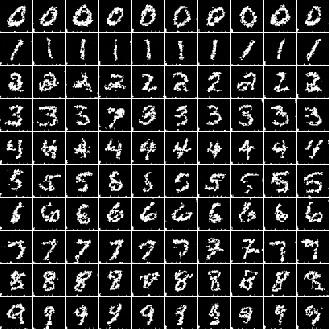
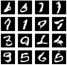
Our output is as follows:
As you can see in Figure 11, the outputs generated by our GAN becomes much more realistic over time.
Congratulations
You have built and trained a generative adversarial network (GAN) model, which can successfully create handwritten digits. There are obviously some samples that are not very clear, but only for 60 epochs trained on only 60,000 samples, I would say that the results are very promising.
Once you can build and train this network, you can generate much more complex images,
- by working with a larger dataset with colored images in high definition;
- by creating a more sophisticated discriminator and generator network;
- by increasing the number of epochs;
- by working on a GPU-enabled powerful hardware
In the end, you can create art pieces such as poems, paintings, text or realistic photos & videos.
Subscribe to the Mailing List for the Full Code
If you would like to have access to full code on Google Colab and have access to my latest content, subscribe to the mailing list: ✉️