

常用概念
边缘计算
之前通常的做法是把数据抓下来,存在到硬盘里,下次需要的时候再拿出来查看。现在新的计算,会实时处理,抛弃无用数据,直接对有效数据进行处理。如果英伟达的GPU,在红绿灯路口,会直接抓取违章等有效数据,不需要的数据直接抛弃。
Deep Learning及成功应用
ML vs DL
Machine Learning:处理 大量的,结构化的,线性的数据
Deep Learning: 处理 video, Image, Speech, Audio
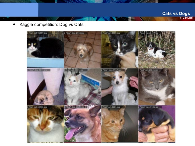
识图 Image Recognition
图片之间差别不大,下面是著名的李飞飞图集,被Google采用

增强学习
李开复的Blue
AlphaGo / Master
Detect pneumothorax in real X-Ray scans
X光扫描结果判定癌症
Audio
声音在时间序列中有很强的相关性。图片在空间中有很强的相关性。
两者采用的深度学习的模型不完全一样
Video / Image -> CNN 卷积 Concurrent
Speech / Audio -> RNN 循环 Recurrent
Vision is Hard
Illumination Variability 光线度

Pose Variability and Occlusions 不同姿势
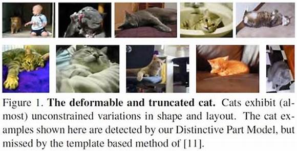
Intra-Class Variability 相似物种
开发实现
各层(库)的实现如下
- H5 + CSS3
- Application (C++, Java, Python)
- STL, site-packages
- Numpy, Pandas, Scipy, Matplot, PIL
- tensorflow
- CUDNN
- CUDA Driver
- CPU & GPU
- MPU (CPU) x86 ARM / GPU NVIDA
- Intel CPU + AMD GPU + DSP + Altera FPGA
- NVIDA ARM CPU + GPU + DSP + Xilinx FPGA
tensorflow
可以识图,工业应用;功能最全,可移植性最强;利于二次开发。
安装
pip3 install tensorflow
pip3 install tensorflow -gpu #可选
python建议用python3,python2虽然支持,但已经不再升级,并且部分功能不支持。python3里建议使用python3.6, python3.7最新的可能不稳定
Hello World
安装完成后,执行下面代码查看tensorflow版本
import tensorflow as tf
tf.__version__
输出结果
'1.11.0'
启动tensorflow
hello = tf.constant("Hello Tensorflow")
sess = tf.Session()
print(sess.run(hello))
输出结果
b'Hello Tensorflow'
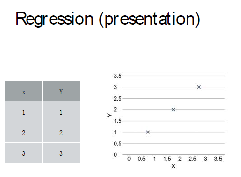
Linear Regression
一维线性感知机
假设有下面这样的X,Y关系,对应的函数关系可能如右图(线性情况下)
但是对于计算机来说,它怎么能知道是这条曲线,它可能预测的为其他两条曲线
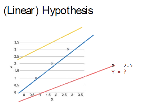
数学的方法是定义一条假设曲线,然后算各个点到它的距离的平方差,最小的那条曲线就是符合条件的那条曲线
公式的验证在原理里有
这条函数我们称之为成本函数
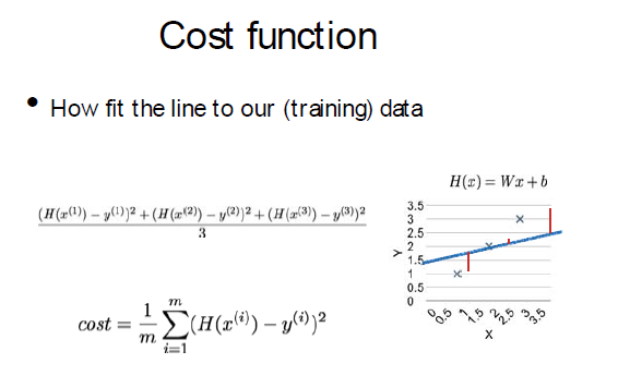
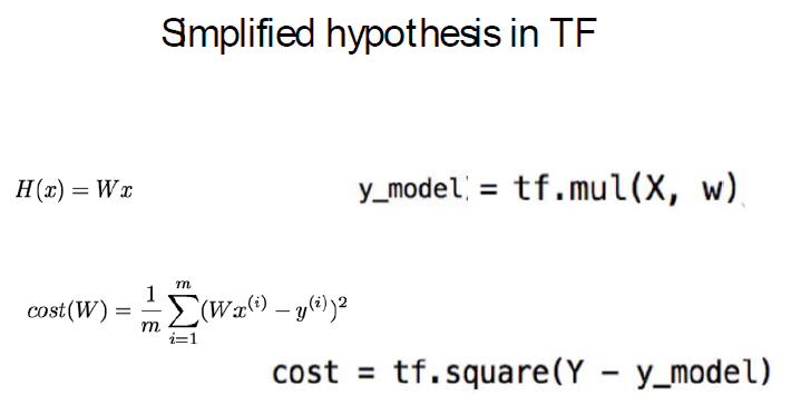
在tensorflow里,这条假设曲线为H(x)/Wx,即y_model=tf.mul(X,w) ,实际点为y
成本cost为cost =tf.square(Y - y_model)
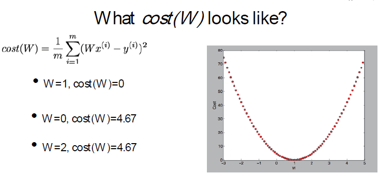
对应的cost曲线如下,可以看到它是一个单调对称曲线,在极点处cost最低,所以可以对W求偏导,在极点处,导数为0,cost最低
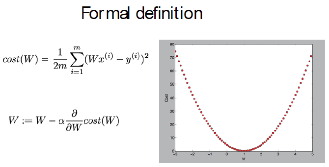
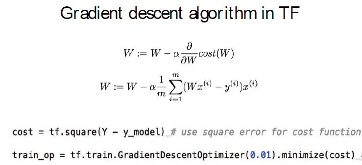
成本函数和W取值对应公式如下,对于W,可以把上面曲线切成无限小,那么每一个切片都是直线,α是这个分割步长。
可以看到越靠近极点,导数越小,W取值越密集,越远离极点,导数越大,W的间隔越大,随着导数的变化不断的调整步长。这个跟我们实际逻辑是完全符号的。
上述梯度下降方法在tensorflow中的实现如下
optimizer = tf.train.GradientDescentOptimizer(learning_rate=0.01)
learning_rate即为步长α,GradientDescentOptimizer表示tensorflow会用梯度下降方法来计算W和cost
下面是完整的代码例子
# X and Y data
x_train = [1, 2, 3]
y_train = [1, 2, 3]

W = tf.Variable(tf.random_normal([1]), name='weight')
b = tf.Variable(tf.random_normal([1]), name='bias')

# Our hypothesis XW+b
hypothesis = x_train * W + b

# cost/loss function
cost = tf.reduce_mean(tf.square(hypothesis - y_train)) # 均方差, reduce_mean (算术平均)

# Minimize
optimizer = tf.train.GradientDescentOptimizer(learning_rate=0.01) #梯度下降
train = optimizer.minimize(cost) # 最小成本

# Launch the graph in a session.
sess = tf.Session()
# Initializes global variables in the graph.
sess.run(tf.global_variables_initializer())
# Fit the line
for step in range(2001):
    sess.run(train)
    if step % 20 == 0:
        print(step, sess.run(cost), sess.run(W), sess.run(b))
简单的代码解释
分为三步
build graph using tensorflow operation
W = tf.Variable(tf.random_normal([1]), name='weight')
b = tf.Variable(tf.random_normal([1]), name='bias')
指定了W和b变量是两个1维向量
hypothesis = x_train * W + b
这个是假设函数,就是我们的Y = Wx + b
cost = tf.reduce_mean(tf.square(hypothesis - y_train)) # 均方差, reduce_mean (算术平均)
成本/损失函数,square调用均方,reduce_mean算法平均,这个跟我们前面的cost函数是一致的
optimizer = tf.train.GradientDescentOptimizer(learning_rate=0.01)
定义梯度下降函数
train = optimizer.minimize(cost)
指定用这个梯度下降函数来算最小cost
run / update graph and get result
sess.run(train)
print(step, sess.run(cost), sess.run(W), sess.run(b))
最后调用sess.run来算它的cost, W和b
查看输出结果
0 2.8683815 [0.04378858] [0.4094853]
20 0.088406585 [0.6464984] [0.6356056]
40 0.057474043 [0.7162222] [0.629098]
60 0.05199197 [0.73461586] [0.6017574]
...
1960 5.5448436e-06 [0.9972651] [0.00621713]
1980 5.036019e-06 [0.9973936] [0.00592493]
2000 4.5740157e-06 [0.9975161] [0.00564648]
cost不断收敛, W趋向去1,b趋向于0
placeholder
如果我们希望在最后可以灵活的输入input数据,而不是一开始就固定,可以用placeholder喂数.
并且这样也能够方便我们验证结果.
import tensorflow as tf
W = tf.Variable(tf.random_normal([1]), name='weight')
b = tf.Variable(tf.random_normal([1]), name='bias')
X = tf.placeholder(tf.float32, shape=[None])
Y = tf.placeholder(tf.float32, shape=[None])
# Our hypothesis XW+b
hypothesis = X * W + b

# cost/loss function
cost = tf.reduce_mean(tf.square(hypothesis - Y))

# Minimize
optimizer = tf.train.GradientDescentOptimizer(learning_rate=0.01)
train = optimizer.minimize(cost)

# Launch the graph in a session.
sess = tf.Session()
# Initializes global variables in the graph.
sess.run(tf.global_variables_initializer())
# Fit the line
for step in range(2001):
    cost_val, W_val, b_val, _ = sess.run([cost, W, b, train],
    feed_dict={X: [1, 2, 3], Y: [1, 2, 3]})
    if step % 20 == 0:
        print(step, cost_val, W_val, b_val)

# Testing our Model
print(sess.run(hypothesis, feed_dict={X:[5]}))
测试结果
2000 2.9081033e-05 [1.0062482] [-0.01420365]

[5.017038]
喂数的话可以通过直接读取文件,下面是一段实例代码
xy = np.loadtext('data.csv', delimiter='', dtype=np.float32)
x_data = xy[:, 0:-1] # 读取不包含最后一列的所有列
y_data = xy[:, [-1]] # 读取最后一列
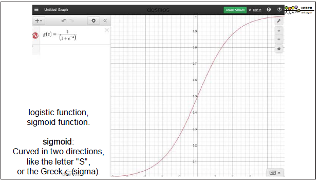
Logistic Regression
逻辑回归
逻辑只有两种结果True和False
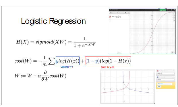
这个结果并不是线性的,我们用下面的曲线来表示这种结果,大于某个阈值时为1,反之为0.一般选用0.5
并且用熵来表示它的成本函数, 公式里y只有1和0两种情况,它仍然是关于W的函数,通过对W求偏导可以得出它的最小成本。
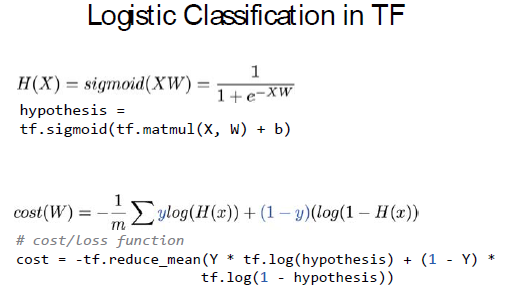
对应的tensorflow如下
完整代码如下
import numpy as np

x_data = np.array([[1, 2], [2, 3], [3, 1], [4, 3], [5, 3], [6, 2]], dtype=np.float32)
y_data = np.array([[0], [0], [0], [1], [1], [1]], dtype=np.float32)

# placeholders for a tensor that will be always fed.
X = tf.placeholder(tf.float32)
Y = tf.placeholder(tf.float32)
W = tf.Variable(tf.random_normal([2, 1]), name='weight')
b = tf.Variable(tf.random_normal([1]), name='bias')

# Hypothesis using sigmoid: tf.div(1., 1. + tf.exp(tf.matmul(X, W) + b))
hypothesis = tf.sigmoid(tf.matmul(X, W) + b)

# cost/loss function
cost = -tf.reduce_mean(Y * tf.log(hypothesis) + (1 - Y) * tf.log(1 - hypothesis))
train = tf.train.GradientDescentOptimizer(learning_rate=0.01).minimize(cost)

# Accuracy computation
# True if hypothesis>0.5 else False
predicted = tf.cast(hypothesis > 0.5, dtype=tf.float32)
accuracy = tf.reduce_mean(tf.cast(tf.equal(predicted, Y), dtype=tf.float32))

# Launch graph
with tf.Session() as sess:
    # Initialize TensorFlow variables
    sess.run(tf.global_variables_initializer())
    for step in range(10001):
        cost_val, _ = sess.run([cost, train], feed_dict={X: x_data, Y: y_data})
        if step % 200 == 0:
            print(step, cost_val)
    # Accuracy report
    h, c, a = sess.run([hypothesis, predicted, accuracy], feed_dict={X: x_data, Y: y_data})
    print("\nHypothesis: ", h, "\nCorrect (Y): ", c, "\nAccuracy: ", a)
结果为
Hypothesis:
 [[0.03148839]
 [0.1598486 ]
 [0.30842718]
 [0.7797612 ]
 [0.93854874]
 [0.9798251 ]]
Correct (Y):
 [[0.]
 [0.]
 [0.]
 [1.]
 [1.]
 [1.]]
Accuracy: 1.0
几个地方说明一下
W = tf.Variable(tf.random_normal([2, 1]), name='weight')
b = tf.Variable(tf.random_normal([1]), name='bias')
这儿W为2X1维度,b为1维
# Hypothesis using sigmoid: tf.div(1., 1. + tf.exp(tf.matmul(X, W) + b))
hypothesis = tf.sigmoid(tf.matmul(X, W) + b)
假设函数为sigmoid
# cost/loss function
cost = -tf.reduce_mean(Y * tf.log(hypothesis) + (1 - Y) * tf.log(1 - hypothesis))
train = tf.train.GradientDescentOptimizer(learning_rate=0.01).minimize(cost)
成本函数为熵,依然用梯度下降方法求cost
# True if hypothesis>0.5 else False
predicted = tf.cast(hypothesis > 0.5, dtype=tf.float32)
accuracy = tf.reduce_mean(tf.cast(tf.equal(predicted, Y), dtype=tf.float32))
预测结果转换为True/False逻辑值
异或
同样的方法,我们来算一下异或
import numpy as np

x_data = np.array([[0, 0], [0, 1], [1, 0], [1, 1]], dtype=np.float32)
y_data = np.array([[0], [1], [1], [0]], dtype=np.float32)

# placeholders for a tensor that will be always fed.
X = tf.placeholder(tf.float32)
Y = tf.placeholder(tf.float32)
W = tf.Variable(tf.random_normal([2, 1]), name='weight')
b = tf.Variable(tf.random_normal([1]), name='bias')

# Hypothesis using sigmoid: tf.div(1., 1. + tf.exp(tf.matmul(X, W) + b))
hypothesis = tf.sigmoid(tf.matmul(X, W) + b)

# cost/loss function
cost = -tf.reduce_mean(Y * tf.log(hypothesis) + (1 - Y) * tf.log(1 - hypothesis))
train = tf.train.GradientDescentOptimizer(learning_rate=0.01).minimize(cost)

# Accuracy computation
# True if hypothesis>0.5 else False
predicted = tf.cast(hypothesis > 0.5, dtype=tf.float32)
accuracy = tf.reduce_mean(tf.cast(tf.equal(predicted, Y), dtype=tf.float32))

# Launch graph
with tf.Session() as sess:
    # Initialize TensorFlow variables
    sess.run(tf.global_variables_initializer())
    for step in range(10001):
        cost_val, _ = sess.run([cost, train], feed_dict={X: x_data, Y: y_data})
        if step % 200 == 0:
            # print(step, cost_val)
            print(step, sess.run(cost, feed_dict={X: x_data, Y: y_data}), sess.run(W))
    # Accuracy report
    h, c, a = sess.run([hypothesis, predicted, accuracy], feed_dict={X: x_data, Y: y_data})
    print("\nHypothesis: ", h, "\nCorrect (Y): ", c, "\nAccuracy: ", a)
结果如下
Hypothesis:
 [[0.502292 ]
 [0.50013524]
 [0.5005841 ]
 [0.49842733]]
Correct (Y):
 [[1.]
 [1.]
 [1.]
 [0.]]
Accuracy: 0.75
可以看到,结果并不能达到100%,因为假设值总是在0.5附近,这是为什么呢?
我们通过电路图来看一下异或门
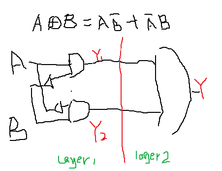
因为异或不是单层逻辑,它有多层。 需要Deep Learninig. 先要得到Y1,Y2,再推出Y.
我们用Neural Network来理解一下这个过程, x,y有四组输入,图中只写了(1,1)这种情况,其他情况同样方法已算好
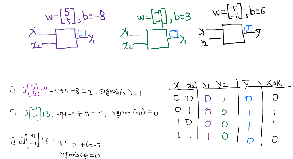
如果我们中间添加一层 W1/b1,那么最后的结果是一致的。
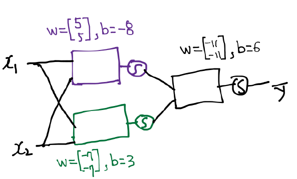
合起来的图效果如上
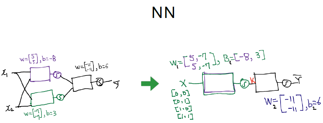
我们将两个W/b进行合并, 变成2*2
增加一层
# X为4*2, W1 2*2 W2 2*1,最终Y为4*1

import numpy as np

x_data = np.array([[0, 0], [0, 1], [1, 0], [1, 1]], dtype=np.float32)
y_data = np.array([[0], [1], [1], [0]], dtype=np.float32)

# placeholders for a tensor that will be always fed.
X = tf.placeholder(tf.float32)
Y = tf.placeholder(tf.float32)

# 第一层
W1 = tf.Variable(tf.random_normal([2, 2]), name='weight1')
b1 = tf.Variable(tf.random_normal([2]), name='bias1')
layer1 = tf.sigmoid(tf.matmul(X, W1) + b1)

# 第二层
W2 = tf.Variable(tf.random_normal([2, 1]), name='weight2')
b2 = tf.Variable(tf.random_normal([1]), name='bias2')
hypothesis = tf.sigmoid(tf.matmul(layer1, W2) + b2)


# cost/loss function
cost = -tf.reduce_mean(Y * tf.log(hypothesis) + (1 -Y) * tf.log(1 -hypothesis))
train = tf.train.GradientDescentOptimizer(learning_rate=0.1).minimize(cost)

# Accuracy computation
# True if hypothesis>0.5 else False
predicted = tf.cast(hypothesis > 0.5, dtype=tf.float32)
accuracy = tf.reduce_mean(tf.cast(tf.equal(predicted, Y), dtype=tf.float32))

# Launch graph
with tf.Session() as sess:
    # Initialize TensorFlow variables
    sess.run(tf.global_variables_initializer())
    for step in range(10001):
        sess.run(train, feed_dict={X: x_data, Y: y_data})
        if step % 100 == 0:
            print(step, sess.run(cost, feed_dict={X: x_data, Y: y_data}), sess.run([W1, W2]))
    # Accuracy report
    h, c, a = sess.run([hypothesis, predicted, accuracy], feed_dict={X: x_data, Y: y_data})
    print("\nHypothesis: ", h, "\nCorrect (Y): ", c, "\nAccuracy: ", a)
结果如下
Hypothesis: [[0.01468208]
 [0.98893714]
 [0.98852473]
 [0.01269323]]
Correct (Y): [[0.]
 [1.]
 [1.]
 [0.]]
Accuracy: 1.0
我们是不是可以做的更好?
堆积网络,让预测值更靠近0和1
方法包括:变得更宽 或者 更深
加宽
# X为4*2, W1 2*10 W2 10*1,最终Y为4*1
import tensorflow as tf
import numpy as np

x_data = np.array([[0, 0], [0, 1], [1, 0], [1, 1]], dtype=np.float32)
y_data = np.array([[0], [1], [1], [0]], dtype=np.float32)

# placeholders for a tensor that will be always fed.
X = tf.placeholder(tf.float32)
Y = tf.placeholder(tf.float32)

# 第一层
W1 = tf.Variable(tf.random_normal([2, 10]), name='weight1')
b1 = tf.Variable(tf.random_normal([10]), name='bias1')
layer1 = tf.sigmoid(tf.matmul(X, W1) + b1)

# 第二层
W2 = tf.Variable(tf.random_normal([10, 1]), name='weight2')
b2 = tf.Variable(tf.random_normal([1]), name='bias2')
hypothesis = tf.sigmoid(tf.matmul(layer1, W2) + b2)


# cost/loss function
cost = -tf.reduce_mean(Y * tf.log(hypothesis) + (1 -Y) * tf.log(1 -hypothesis))
train = tf.train.GradientDescentOptimizer(learning_rate=0.1).minimize(cost)

# Accuracy computation
# True if hypothesis>0.5 else False
predicted = tf.cast(hypothesis > 0.5, dtype=tf.float32)
accuracy = tf.reduce_mean(tf.cast(tf.equal(predicted, Y), dtype=tf.float32))

# Launch graph
with tf.Session() as sess:
    # Initialize TensorFlow variables
    sess.run(tf.global_variables_initializer())
    for step in range(10001):
        sess.run(train, feed_dict={X: x_data, Y: y_data})
        if step % 100 == 0:
            print(step, sess.run(cost, feed_dict={X: x_data, Y: y_data}), sess.run([W1, W2]))
    # Accuracy report
    h, c, a = sess.run([hypothesis, predicted, accuracy], feed_dict={X: x_data, Y: y_data})
    print("\nHypothesis: ", h, "\nCorrect (Y): ", c, "\nAccuracy: ", a)
结果如下
Hypothesis:
 [[0.00463089]
 [0.99264306]
 [0.9913278 ]
 [0.01108391]]
Correct (Y):
 [[0.]
 [1.]
 [1.]
 [0.]]
Accuracy: 1.0
假设值离0和1更近了
加深
# X为4*2, W1 2*10 W2 10*10 W3 10*10 W4 10*1,最终Y为4*1
import tensorflow as tf
import numpy as np

x_data = np.array([[0, 0], [0, 1], [1, 0], [1, 1]], dtype=np.float32)
y_data = np.array([[0], [1], [1], [0]], dtype=np.float32)

# placeholders for a tensor that will be always fed.
X = tf.placeholder(tf.float32)
Y = tf.placeholder(tf.float32)

# 第一层
W1 = tf.Variable(tf.random_normal([2, 10]), name='weight1')
b1 = tf.Variable(tf.random_normal([10]), name='bias1')
layer1 = tf.sigmoid(tf.matmul(X, W1) + b1)

# 第二层
W2 = tf.Variable(tf.random_normal([10, 10]), name='weight2')
b2 = tf.Variable(tf.random_normal([10]), name='bias2')
layer2 = tf.sigmoid(tf.matmul(layer1, W2) + b2)

# 第三层
W3 = tf.Variable(tf.random_normal([10, 10]), name='weight3')
b3 = tf.Variable(tf.random_normal([10]), name='bias3')
layer3 = tf.sigmoid(tf.matmul(layer2, W3) + b3)

# 第四层
W4 = tf.Variable(tf.random_normal([10, 1]), name='weight4')
b4 = tf.Variable(tf.random_normal([1]), name='bias4')
hypothesis = tf.sigmoid(tf.matmul(layer3, W4) + b4)

# cost/loss function
cost = -tf.reduce_mean(Y * tf.log(hypothesis) + (1 -Y) * tf.log(1 -hypothesis))
train = tf.train.GradientDescentOptimizer(learning_rate=0.1).minimize(cost)

# Accuracy computation
# True if hypothesis>0.5 else False
predicted = tf.cast(hypothesis > 0.5, dtype=tf.float32)
accuracy = tf.reduce_mean(tf.cast(tf.equal(predicted, Y), dtype=tf.float32))

# Launch graph
with tf.Session() as sess:
    # Initialize TensorFlow variables
    sess.run(tf.global_variables_initializer())
    for step in range(10001):
        sess.run(train, feed_dict={X: x_data, Y: y_data})
        if step % 100 == 0:
            print(step, sess.run(cost, feed_dict={X: x_data, Y: y_data}), sess.run([W1, W2, W3, W4]))
    # Accuracy report
    h, c, a = sess.run([hypothesis, predicted, accuracy], feed_dict={X: x_data, Y: y_data})
    print("\nHypothesis: ", h, "\nCorrect (Y): ", c, "\nAccuracy: ", a)
结果如下
Hypothesis:
 [[0.00208044]
 [0.99804413]
 [0.9964066 ]
 [0.00284347]]
Correct (Y):
 [[0.]
 [1.]
 [1.]
 [0.]]
Accuracy: 1.0
运行的时间更长了,结果也更加精确。那么可以无限加宽吗?不行,会造成过拟合
过拟合 overfitting,过于严格的比对,反而导致无法判断结果
如果把上例改成10层,那么结果反而不收敛
解决overfitting可以用:
- Regularization Dropout : 打掉一些相关性低的点,否则反向导数级数太深 - 可以用ReLu代替sigmod进行线性整流
- Early Stop : 如果accurate不再提高,可以停止拟合
ReLU: Rectified Linear Unit
整流 - 解决overfitting问题, >=0, self; < 0, 0; 打掉偏差大的点
使用ReLU之后,即使增加到10层,依然工作
softmax
处理多标签
tensorboard
tensorflow安装时,它会自动安装
启动命令为
tensorboard --logdir=./logs
Tesorboard的使用分5部
- which tensors you want to log
w2_hist = tf.summary.histogram("weights2", W2)
cost_summ = tf.summary.scalar("cost", cost)
- Merge all summaries
summary= tf.summary.merge_all()
- Create writer and add graph
# Create summary writer
writer = tf.summary.FileWriter(‘./logs’)
writer.add_graph(sess.graph)
- Run summary merge and add_summary
s, _ = sess.run([summary, optimizer], feed_dict=feed_dict)
writer.add_summary(s, global_step=global_step)
- Launch TensorBoard
tensorboard --logdir=./logs
前面的异或逻辑回归的例子修改后的代码如下
# Lab 9 XOR
import tensorflow as tf
import numpy as np

tf.set_random_seed(777) # for reproducibility
learning_rate = 0.01

x_data = [[0, 0],
          [0, 1],
          [1, 0],
          [1, 1]]
y_data = [[0],
          [1],
          [1],
          [0]]
x_data = np.array(x_data, dtype=np.float32)
y_data = np.array(y_data, dtype=np.float32)

# X = tf.placeholder(tf.float32)
# Y = tf.placeholder(tf.float32)

X = tf.placeholder(tf.float32, [None, 2], name='x-input')
Y = tf.placeholder(tf.float32, [None, 1], name='y-input')

with tf.name_scope("layer1"):
    W1 = tf.Variable(tf.random_normal([2, 2]), name='weight1')
    b1 = tf.Variable(tf.random_normal([2]), name='bias1')
    layer1 = tf.sigmoid(tf.matmul(X, W1) + b1)
#
    w1_hist = tf.summary.histogram("weights1", W1)
    b1_hist = tf.summary.histogram("biases1", b1)
    layer1_hist = tf.summary.histogram("layer1", layer1)

with tf.name_scope("layer2"):
    W2 = tf.Variable(tf.random_normal([2, 1]), name='weight2')
    b2 = tf.Variable(tf.random_normal([1]), name='bias2')
    hypothesis = tf.sigmoid(tf.matmul(layer1, W2) + b2)
#
    w2_hist = tf.summary.histogram("weights2", W2)
    b2_hist = tf.summary.histogram("biases2", b2)
    hypothesis_hist = tf.summary.histogram("hypothesis", hypothesis)


# cost/loss function
with tf.name_scope("cost"):
    cost = -tf.reduce_mean(Y * tf.log(hypothesis) + (1 - Y) *
                           tf.log(1 - hypothesis))
    cost_summ = tf.summary.scalar("cost", cost)

with tf.name_scope("train"):
    train = tf.train.AdamOptimizer(learning_rate=learning_rate).minimize(cost)

# Accuracy computation
# True if hypothesis>0.5 else False
predicted = tf.cast(hypothesis > 0.5, dtype=tf.float32)
accuracy = tf.reduce_mean(tf.cast(tf.equal(predicted, Y), dtype=tf.float32))
accuracy_summ = tf.summary.scalar("accuracy", accuracy)

# Launch graph
with tf.Session() as sess:
    # tensorboard --logdir=./logs/xor_logs
    merged_summary = tf.summary.merge_all()
    writer = tf.summary.FileWriter("./logs/xor_logs_r0_01")
    writer.add_graph(sess.graph) # Show the graph
    # Initialize TensorFlow variables
    sess.run(tf.global_variables_initializer())
    for step in range(10001):
        summary, _ = sess.run([merged_summary, train], feed_dict={X: x_data, Y: y_data})
        writer.add_summary(summary, global_step=step)
        if step % 100 == 0:
            print(step, sess.run(cost, feed_dict={
                  X: x_data, Y: y_data}), sess.run([W1, W2]))
    # Accuracy report
    h, c, a = sess.run([hypothesis, predicted, accuracy],
                       feed_dict={X: x_data, Y: y_data})
    print("\nHypothesis: ", h, "\nCorrect: ", c, "\nAccuracy: ", a)


'''
Hypothesis: [[ 6.13103184e-05]
 [ 9.99936938e-01]
 [ 9.99950767e-01]
 [ 5.97514772e-05]]
Correct: [[ 0.]
 [ 1.]
 [ 1.]
 [ 0.]]
Accuracy: 1.0
'''

评论
留言请先登录或注册! 并在激活账号后留言!